Application of Cofactor Expansion

Laplace expansion, also known as cofactor expansion or first Laplace theorems on determinants, is a recursive way to calculate determinant of a square matrix.

But it’s also clear that for a generic matrix, using cofactor expansion is much slower than using LU decomposition. So, what’s the real advantage of Laplace expansion? In what kind of situation can we use this method?

To give a quick answer: when a matrix comes with many zeros.

Additionally, when a matrix constitutes some variables.

From the Definition

Besides expressing the theorem with sigma notaion (Σ), there is also another equivalent form accroding to Linear Algebra for Computational Sciences and Engineering:

The determinant of a matrix is equal to scalar product of a row (column) vector by the corresponding vector of cofactors.

I rather like this definition.

Being Lazy

We can note that each term of summation is the product of a matrix entry and its cofactor.

So, it’s clear that if any of the two factors is zero, this term will be zero and we can calculate one thing less.

Although an entry’s cofactor needs some complex arithmetic, zero entries in a matrix can be easily determined.

Handling Some Uncertainty

Thinking from the opposite, lower-upper decomposition is probably not completely applicable to a matrix with some variables. In this case, we cannot determine an entry is a pivot or not if it contain some unknowns.

At this point, cofactor expansion can help, but this is not the focus of this post.

Real Stuff

Let’s realize it in Python and check what outcome exactly could be when there are some zeros in a matrix.

Reinvent the Wheel

Firstly, we need to gengerate a square matrix randomly.

Generate a Matrix

import random

def square_matrix_gen(n, a, b, zeros=0):
    m = []
    for i in range(n):
        row = []
        for j in range(n):
            entry = int(random.uniform(a, b))
            if entry == 0:
                if zeros == 0:
                    while (entry == 0):
                        entry = int(random.uniform(a, b))
                if zeros > 0:
                    zeros = zeros -1
            row.append(entry)
        m.append(row)
    while zeros != 0:
        i = int(random.randrange(n))
        j = int(random.randrange(n))
        if m[i][j] != 0:
            m[i][j] = 0
            zeros = zeros -1
    return m

def print_matrix(m):
    n = len(m)
    for i in range(n):
        for j in range(n):
            print(m[i][j], end='\t')
        print()

In Line 8, int(random.uniform(lower, upper)) returns a value in continuous uniform distribution. Bounds lower and upper are not included since there is a type cast with int().

Note that 0 is also in the bounds, so from Line 9 to Line 14 we are handling this problem, trying to make sure that the number of zeros in the returned matrix is exactly the same as zeros we passed in. This may demolish the idea of uniform distribution, but not impact the purpose of this demonstration.

A = square_matrix_gen(3, -100, 100)
print_matrix(A)

B = square_matrix_gen(5, -100, 100, 4)
print_matrix(B)

Output (probably):

-11     -9      -89
39      44      72
-96     -14     70

-14     0       -99     47      0
0       7       18      85      -66
66      66      30      -4      4
-98     12      -83     20      0
-21     15      48      1       -93

Realization

To calculate determinant, according to cofactor expansion, we need cofactor. As for cofactor, we need complement minor, which comes from complement submatrix.

def det(m):
    n = len(m)
    if n == 0:
        raise ValueError
    elif n == 1:
        return m[0][0]
    i = int(random.randrange(n))
    summation = 0
    for j in range(n):
        if m[i][j] != 0:
            summation += m[i][j] * cofactor(m, i, j)
    return summation

def cofactor(m, i, j):
    co = (-1) ** (i + j) * complement_minor(m, i, j)
    return co

def complement_minor(m, i, j):
    submatrix = complement_submatrix(m, i, j)
    minor = det(submatrix)
    return minor

def complement_submatrix(m, i, j):
    n = len(m)
    sub = m[:i] + m[i+1:]
    for x in range(n-1):
        sub[x] = sub[x][:j] + sub[x][j+1:]
    return sub

Complement minor is exactly the determinant of complement submatrix, so the sequence of function call expands in a recursive manner.

In Line 7, we selected a random row to apply first Laplace theorem. Note that all rows and columns begin with 0 index and end with n-1.

Function of complement submatrix is a little bit fancy. Essentially, it’s just a bunch of list slicing.

Benchmarking

Cofactors are useful when matrices have many zeros.

Gilbert Strang, Introduction to Linear Algebra

To test its convenience, we can simply measure running time it used.

from datetime import datetime

print('Num of zeros\tTime used')

for i in range(10, 26):
    m = square_matrix_gen(10, -100, 100, i)
    t1 = datetime.now()
    det(m)
    t2 = datetime.now()
    print(f'{i}\t\t{t2-t1}')

Output:

Num of zeros    Time used
10              0:00:04.076951
11              0:00:03.756362
12              0:00:02.944325
13              0:00:02.906601
14              0:00:02.848988
15              0:00:02.384444
16              0:00:02.215670
17              0:00:02.151262
18              0:00:02.014808
19              0:00:01.391330
20              0:00:01.436479
21              0:00:01.417628
22              0:00:01.162688
23              0:00:00.958879
24              0:00:01.125304
25              0:00:00.949000

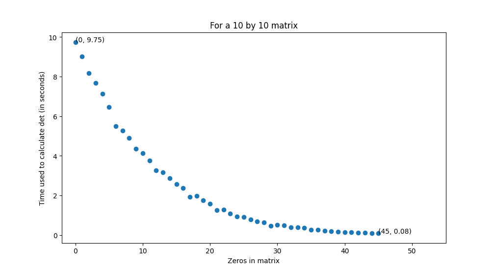
We can see that with the number of zeros in matrix increase, time needed to calculate det() is getting less rapidly.

Here is a result in terms of a 10 by 10 matrix with number of zeros ranging from 0 to 45, plotted with matplotlib.pyplot (for full script, please refer to Appendix):

From Figure 1 we can see that only a few zeros can reduce calculation time to a large extend.

Here we just pick a random row to calculate det(), and if we chose a row (column) with the most zeros, the time might have been reduced even faster.

Remark

When learning linear algebra and going through the textbook, tons of jargons come in, with many definitions, theorems, proofs and properties. But as a student major in computer science, I really want to know what’s the usage of them, in what circumstances can we use them. I care more about real-life application and realization.

In terms of cofactor expansion, to calculate determinant recursively is a fun topic, but not a very efficient manner, as recursion always occupy a large amount of memory and hard to optimize.

So does almost every industrial implementation of determinant come from LU decomposition.

However, Laplace expansion is not meaningless, and that’s why I wrote this post.

References

1. Linear Algebra for Computational Sciences and Engineering, 2nd Edition, Ferrante Neri, Springer Cham, 2019.
2. Introduction to Linear Algebra, 5th Edition, Gilbert Strang, Wellesley-Cambridge Press, 2016.
3. Cofactor Expansions
4. Laplace expansion - Wikipedia
5. Applications of minors and cofactors
6. LU decomposition - Wikipedia
7. LU Factorization
8. Mutable Sequence Types - Built-in Types - Python 3.11.1 documentation
9. numpy.linalg.det — NumPy v1.24 Manual

Appendix: Full Script

import random
from datetime import datetime
import matplotlib.pyplot as plt

def square_matrix_gen(n, a, b, zeros=0):
    m = []
    for i in range(n):
        row = []
        for j in range(n):
            entry = int(random.uniform(a, b))
            if entry == 0:
                if zeros == 0:
                    while (entry == 0):
                        entry = int(random.uniform(a, b))
                if zeros > 0:
                    zeros = zeros -1
            row.append(entry)
        m.append(row)
    while zeros != 0:
        i = int(random.randrange(n))
        j = int(random.randrange(n))
        if m[i][j] != 0:
            m[i][j] = 0
            zeros = zeros -1
    return m

def print_matrix(m):
    n = len(m)
    for i in range(n):
        for j in range(n):
            print(m[i][j], end='\t')
        print()

def det(m):
    n = len(m)
    if n == 0:
        raise ValueError
    elif n == 1:
        return m[0][0]
    i = int(random.randrange(n))
    summation = 0
    for j in range(n):
        if m[i][j] != 0:
            summation += m[i][j] * cofactor(m, i, j)
    return summation

def cofactor(m, i, j):
    co = (-1) ** (i + j) * complement_minor(m, i, j)
    return co

def complement_minor(m, i, j):
    submatrix = complement_submatrix(m, i, j)
    minor = det(submatrix)
    return minor

def complement_submatrix(m, i, j):
    n = len(m)
    sub = m[:i] + m[i+1:]
    for x in range(n-1):
        sub[x] = sub[x][:j] + sub[x][j+1:]
    return sub

def timedelt_to_seconds(t):
    return t.seconds + t.microseconds / 1000000

index = []
time = []
for i in range(46):
    m = square_matrix_gen(10, -100, 100, i)
    t1 = datetime.now()
    det(m)
    t2 = datetime.now()
    tdelt = t2 - t1
    time.append(timedelt_to_seconds(tdelt))
    index.append(i)

for xy in zip([index[0], index[-1]], [time[0], time[-1]]):
    # draw coordinates of the first and last points
    plt.annotate('(%d, %.2f)' % xy, xy=xy)

plt.plot(index, time, 'o')
plt.title('For a 10 by 10 matrix')
plt.xlabel('Zeros in matrix')
plt.ylabel('Time used to calculate det (in seconds)')
plt.xlim([-2, 55])
plt.show()